Uniswap Protocol Fee Report

Introduction

The tradeoffs of protocol fees on Uniswap have been a topic of active debate for several years. Charging LPs a percentage fee for the yield they accrue on Uniswap could be a substantial source of revenue for the protocol, which could then be used to fund various strategic initiatives. On the other hand, there are also significant costs that have so far been difficult to quantify.

To make the best community decision, UNI holders must be equipped with robust research and predictive analysis to better understand the range of outcomes. This report builds on our prior work on DEX economics with the Uniswap Foundation to consider the tradeoffs of protocol fees. We provide estimates of the risks and benefits of implementing a fee to help inform discussions in the community on this important strategic tradeoff.

Background

What is a protocol fee?

Every time someone does a trade on Uniswap, they pay a small fee to the pool’s LPs (liquidity providers). If a protocol fee were turned on, then a small percentage of the trading fee that currently goes to LPs will go to Uniswap instead. So if a protocol fee is implemented, trading won’t get more expensive, but LPing will become less profitable.

What are the advantages of a protocol fee?

Despite the success of Uniswap, the Uniswap protocol doesn’t currently receive any revenue from Uniswap trading activity. The revenue gained from a protocol fee could be put to a productive use by Uniswap governance.

What are the disadvantages of a protocol fee?

A protocol fee would mean that LPs get less yield, which would likely cause some of them to withdraw liquidity. Less liquidity in Uniswap pools means higher slippage for traders: a trader trying to swap USDC for ETH would receive less ETH for a given amount of USDC they put in, because the size of their trade is larger relative to the tokens supplied in the pool by LPs. Because the slippage is higher, traders may decide to use one of Uniswap’s competitors instead. This would result in a decrease in trading volume sent to Uniswap.

Goals

We use economic models and simulations of Uniswap and competing DEXs to evaluate the impact of fees on Uniswap V3 in three different areas:

1. Quantifying the potential benefits of a protocol fee

• How much revenue can a protocol fee generate?

2. Quantifying the potential downsides of a protocol fee

• How much liquidity and volume would be lost, and to what degree should losses be tolerated?

3. Assessing the impact of a protocol fee across different pools

• Are some pools disproportionately affected?

In answering these questions, we take into account many critical details, such as the possibility of triggering negative feedback loops in user response, the different user types and pools on Uniswap, and the dynamics of competing exchanges that may attract cost-sensitive users. However, we do not look to propose a specific protocol fee solution in this report. Since the optimal tradeoff involves many qualitative and strategic factors, we will not make any concrete recommendations until we can further evaluate these in the context of the analysis presented here. Instead, we will focus on forecasts that can help clarify the pros and cons and inform further discussions.

Methodology

To understand how users would react to a fee switch, we built a simulation that predicts how a protocol fee would influence LPs and traders on the per-swap level. This simulation was run on historical Ethereum Uniswap V3 data to project counterfactual liquidity and volume had the fee switch been turned on.

The models used in this report are the latest iteration of tooling that has evolved throughout our work with the Uniswap Foundation. The liquidity-volume model initially developed for incentive analysis is combined with the swap simulator from our more recent work on price execution. This combination allows us to explore detailed counterfactuals within a robust economic framework for how a DEX operates at a higher level.

Liquidity Model

To estimate a range of possible outcomes, we model liquidity through two approaches. The perfect elasticity model represents an upper bound on the reaction LPs would have in response to a drop in yield, and the empirical elasticity model represents a reasonable lower bound.

Perfect Elasticity Model

We conservatively estimate the effects of a protocol fee on liquidity through a perfect elasticity model. If a protocol fee were levied, the yield LPs earn would instantaneously decrease. In response, LPs may start withdrawing liquidity. This would cause the yield that remaining LPs are earning to start increasing, because the fees distributed per unit of liquidity is higher assuming the pool volume hasn't yet changed. Eventually, enough liquidity would be withdrawn to restore the LP yield to the market rate it was at before the protocol fee. This dynamic is illustrated in the figure below.

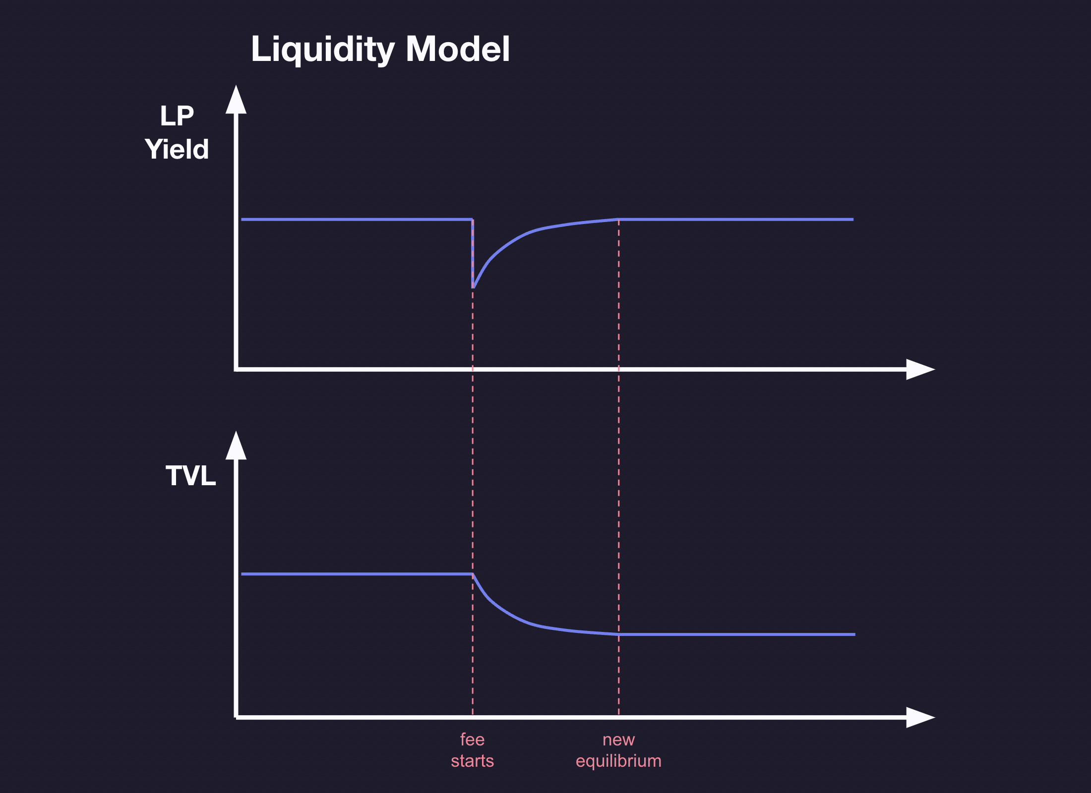
Under this modeling assumption, an X% protocol fee would result in an X% reduction in pool liquidity. It is possible that some LPs would accept a lower APY or adjust their liquidity to a tighter range to return to a higher APY instead of withdrawing. Either of these cases would result in less TVL being removed to restore market equilibrium than we estimate. However, these would also imply that either the efficient level of APY or users' tolerance for impermanent loss has changed. To make our estimates more conservative and avoid excessive assumptions on LP behavior, we exclude changes in LP yield preferences and tick ranges from the impact forecasts. This means that, to a first order, the liquidity model estimates a linear impact of 1% TVL drop uniformly across the tick distribution for every 1% of protocol fee.

Empirical Elasticity Model

Our perfect elasticity assumption only applies in a world of perfect information and frictionless rebalancing. In the real world, LPs are often slow to react to changes in yield and are not constantly rebalancing their liquidity portfolio to match the market rate yield (which itself may not be known with certainty). A different approach would be to use historic yield and liquidity data for the highest-volume pools that have complete data and fit a time series regression model that estimates the impact of past yield and past liquidity on present liquidity. We can specify the model in a way that the values of the regression coefficients provide us with estimates for the short-term elasticity of liquidity in a pool with respect to changes in the yield that an LP can earn from the pool.

We fit a model with the following functional form:

$$\log L_t = \alpha + \beta \log Y_{t-1} + \gamma \log L_{t-1} $$

Where \(L\) is active pool liquidity and \(Y\) is pool yield. In this model, we use the yield and liquidity from previous periods to predict the liquidity in the current period for each pool separately. In this equation, the coefficient \(\beta\) represents the elasticity of liquidity with respect to yield. We also find that the model that fits the data best is one where the lag between periods is 7 days. Applying these models to the 10 pools with the highest volume, we obtain the following results:

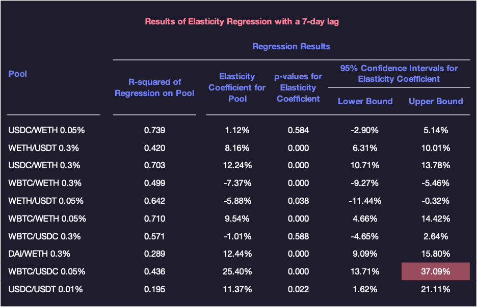
The elasticities estimated for each pool using this model are far lower than the 100% assumed under perfect elasticity. Possible reasons for this lower elasticity are: some LPs might be willing to accept a lower APY; others might adjust their liquidity to a tighter range to return to a higher APY instead of withdrawing; LPs may be slower to react to short-term changes; etc.

At the same time, while this model makes fewer assumptions about the rationality of LPs, it still assumes that their behavior when faced with day-to-day yield changes will extend to a situation where they are faced with a protocol fee instituted from above. Research by behavioral economists has shown that people do not respond symmetrically when faced with symmetric situations, and the institution of the fee is likely to evoke emotive as well as rational responses from LPs. Taking a conservative approach, we look at the pool with the highest point estimate of elasticity, and then take the upper bound of the 95% confidence interval for that estimate. In this case, the estimate chosen is 37.09%, which is the upper bound of the estimate for the WBTC/USDC 0.05% pool. Using this figure in our calculations allows us to say with a high degree of confidence that the actual elasticity is lower than our estimate.

Combining the information from both these approaches, we estimate that the first-order impact of every 1% of an instituted protocol fee would lead to a uniform drop in TVL across the tick distribution that ranges from 0.037% to 1%.

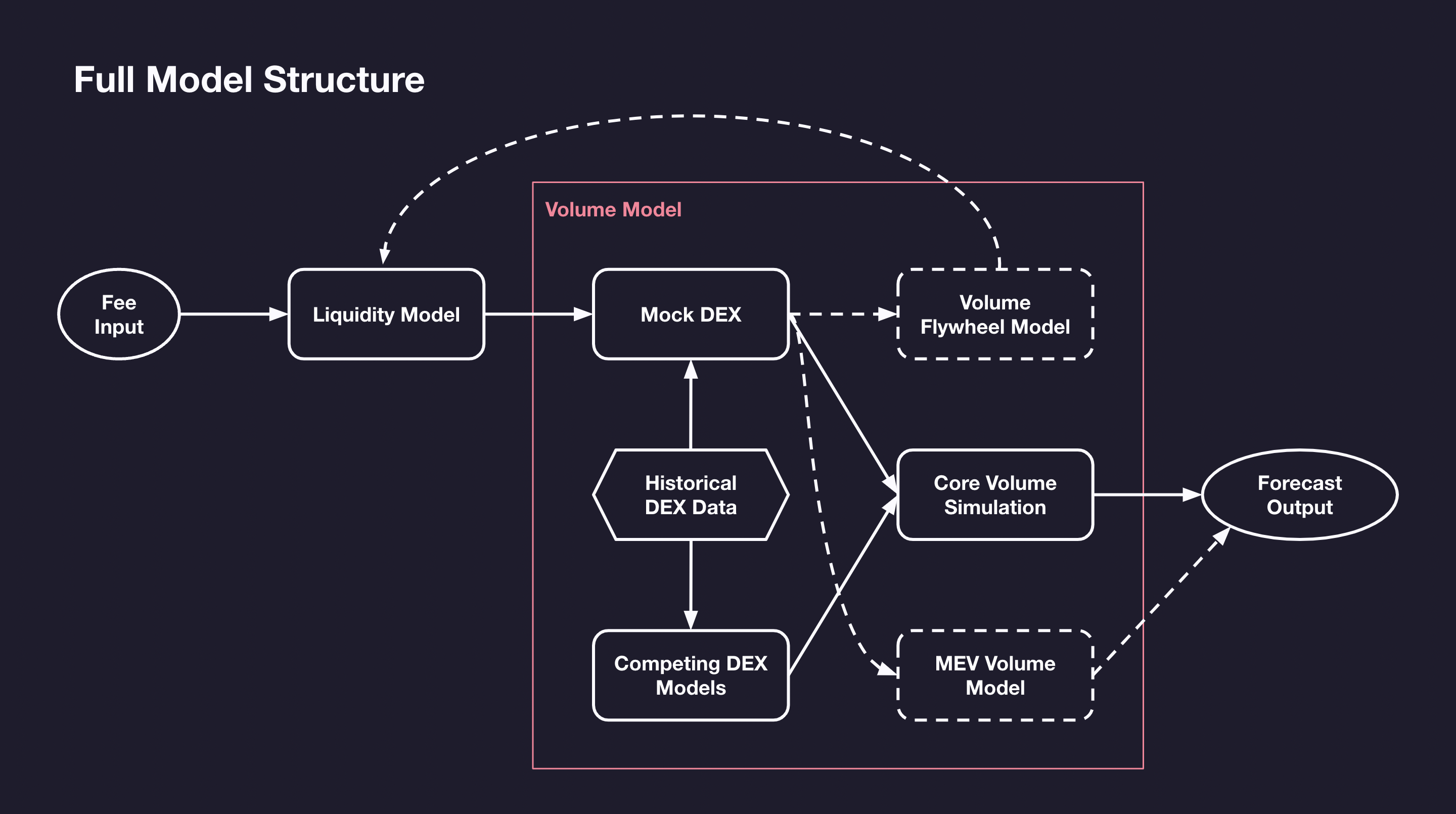
Volume Model

The volume model uses the results from the liquidity model to create a counterfactual DEX pool, called the Mock DEX, within our swap simulator. The simulator can then backtest swaps that were originally routed to the real Uniswap pool on the Mock DEX and competing DEXs. By observing the performance of the Mock DEX in this realistic environment, we can then estimate how much volume would be lost due to its reduced competitiveness caused by the protocol fee.

The diagram shows the component parts of the volume model and how it fits together with the liquidity model. In the following sections, we will break down each of these parts, starting with the core volume simulation.

Core Volume Simulation

The core volume methodology is extended from our earlier Price Execution Analysis, with the addition of the Mock DEX allowing us to explore counterfactual liquidity coonditions as a result of the protocol fee. For each competing DEX, we replicate the precise liquidity conditions at the time of each swap and the specific DEX pool logic that generates the swap output. Based on the simulated swap outputs, we can then identify which swaps would be re-routed if the real Uniswap pool were replaced with the Mock DEX.

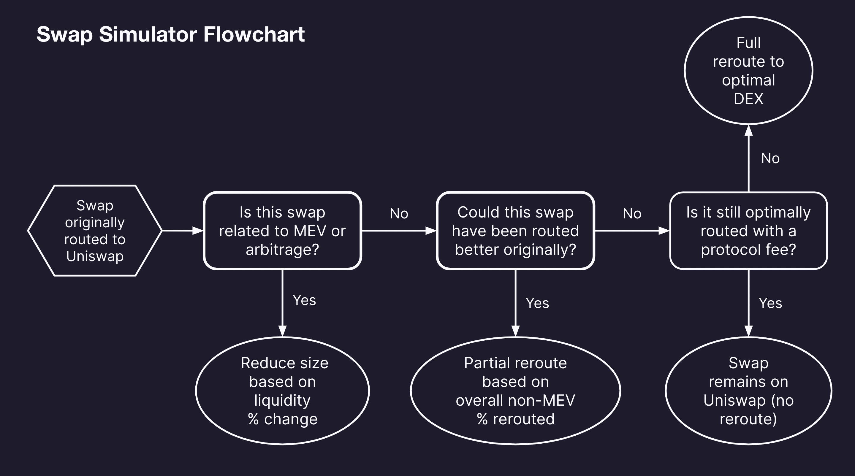
Since we have observed in prior work on incentive design that onchain order routing is very efficient, we generally assume that swaps are routed to the DEX that provides the best swap output, with a few notable exceptions that we will discuss shortly. A typical swap simulation in the model would proceed as shown in the diagram below.

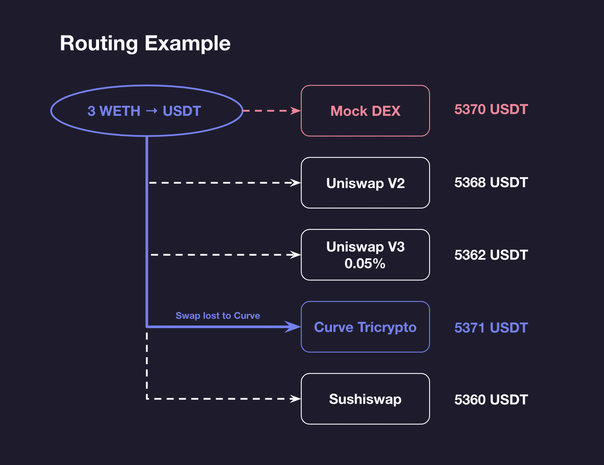
The example shows a real swap in the WETH / USDT 0.3% pool that was re-routed by the swap simulator. Though the swap was optimally executed in the actual WETH / USDT 0.3% pool, the lower liquidity version in the Mock DEX would no longer be the optimal venue. The simulation routing logic then removed this swap from the post-fee volume estimate.

MEV Volume Model

One of the core assumptions in the volume simulation is that the existence of volume is exogenous to liquidity, meaning that if price execution were better at a competitor, that volume would be re-routed to that competitor versus not existing at all. This assumption is violated for MEV volume: MEV traders have a different role in DEX economics and must be modeled more robustly through economic-based estimates than via direct simulation, so we treat them separately in the volume model.

A large proportion of MEV trades are arbitrage, either between two DEXes or between a DEX and a CEX. Arbitrage trades take advantage of price discrepencies between a given pool and another liquidity source, which typically arise from a pool offering a stale price.

If there is a mismatch between a Uniswap V3 pool’s price (p_p) and the market price (p_m) for a given trading pair, the formula below gives us the swap size needed to correct the price discrepency, assuming the swap stays within the current tick bucket with liquidity L:

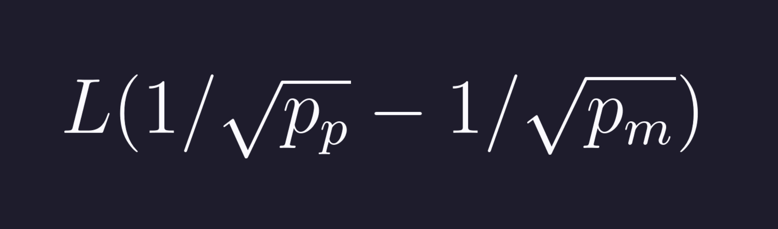
Therefore, the size of an arbitrage trade would decrease proportionally to the pool’s current tick liquidity. As our liquidity model reduces all ticks uniformly, we reduce arbitrage trade volume by the same percentage. Within the context of our historical swap simulation, arbitrage opportunities that existed without a protocol fee would still exist if a protocol fee were levied, but the size of the trade must be updated. Notably, this does not represent a re-routing of arbitrage volume to competing DEXs, but a drop in arbitrage activity overall due to a reduction in opportunities.

Not all MEV trades are arbitrage: we expect some forms of MEV, such as liquidations, to be routed optimally the same way that Core Volume swaps are. But as discussed further in this report, the effect of liquidity loss on arbitrage volume is much greater than the effect on core volume in most cases. Due to the complexity associated with fully modeling the full spectrum of MEV strategies, we make a conservative assumption that all MEV trades are arbitrage trades in our volume model.

In our earlier User Cohort Analysis, we identified MEV trades and noted that they make up between 40 and 80% of volume on Uniswap and other major DEXs. In this analysis, we found that MEV volume is much more sensitive to liquidity than core users, which provides empirical justification to our treatment of MEV volume as arbitrage trades.

Toxicity of MEV Volume

In contrast to retail and institutional (ie. core) volume, which is typically profitable for LPs, MEV volume is highly selective for liquidity at slightly inefficient price ticks and often comes at a cost to LPs who were traded against. This effect is known as “Order Toxicity” and is discussed in much more detail in our incentive design research.

The loss that LPs incur from MEV trades is best illustrated through the concept of LVR (“loss versus rebalancing”) or impermanent loss. If the Uniswap V3 ETH/USDC 0.05% pool were quoting the price of ETH at $2000, but the market price of ETH increased to $2100, then we would expect an arbitrage trade to occur that corrects this price discrepency. Suppose an LP had deposited equal valued amounts of ETH and USDC right before this arbitrage trade, and then withdrew all their liquidity right after. The value of the ETH and USDC they withdrew would be less than the value of the initial portfolio they started with (1 ETH and $2000 USDC) due to the mechanics of how AMMs like Uniswap V3 work (note that the magnitude of this loss would depend on the price range they provided liquidity for). This loss in value incurred is called impermanent loss. Relatedly, LVR is the opportunity cost that the LP faced against an alternative scenario of rebalancing their portfolio when the price changed. Due to these losses, arbitrage trades are generally unprofitable for LPs to receive.

While arbitrage trades could in theory be done by retail traders and look like core volume, they are always done by MEV bots in practice. And while there are other forms of MEV other than arbitrage, we made the conservative assumption in the previous section that all MEV trades are performing arbitrage. As such, we provide separate analysis for MEV and Core volume, as MEV volume is mostly toxic and thus unfavorable for LPs, while Core volume is mostly non-toxic and represents the main end users of the protocol (retail and institutional traders).

Non-Optimal Swaps

For completeness, another edge case to note are swaps that were not optimally routed to begin with. Though the amount of inefficient volume on DEXs is low, there will always be some cases due to noise and unaware traders. For example, in our Price Execution Analysis, we found that about 83% of volume on Uniswap V3 was optimally routed, which leaves 17% as non-optimal trades. In the simulation, we re-route this volume in proportion to the overall reduction of core volume, since most of it likely originates from retail traders who are relatively indifferent to price execution. The full routing logic, including MEV volume and non-optimal swaps, is shown in the diagram below.

Flywheel Effects

Though we have treated them as a one-way linkage so far, volume and liquidity are interdependent and may exhibit feedback channels that amplify the effects of falling activity. Consider the following scenario:

1. A protocol fee is introduced, which cuts the yield that LPs earn
2. LPs start withdrawing their liquidity, which worsens the slippage traders experience
3. Volume decreases, which lowers the fee yield paid to LPs
4. LPs withdraw their liquidity even further, which further worsens the slippage that traders experience
5. Volume decreases further, which causes liquidity to decrease further, repeating in a cycle until some equilibrium is reached

This would be the opposite of the beneficial flywheel that comes up in our work on liquidity mining. To account for the potential downside scenario, we include a feedback mechanism that adjusts the APY in the liquidity model based on the change in core volume. We do so by directly modeling this cycle in our simulation: drops in LP yield as estimated by the volume model are fed back into the liquidity model, which is fed into our volume model to produce new estimates of volume loss, which is repeated until an equilibrium is reached.

Impact Results

Our analysis uses swap and liquidity data on Ethereum Uniswap V3 from August 2023 to January 2024. Our analysis focuses on the pools that are currently charged an interface fee by Uniswap Labs, namely pools swapping between ETH, WBTC, and major stablecoins (USDC, USDT, DAI, agEUR, GUSD, LUSD, EUROC, XSGD), which we refer to as whitelisted pools.

The table below shows the predicted effect of different protocol fees on all the whitelisted pools. We provide lower and upper bound estimates of protocol fee impact, where lower estimates come from the empirical elasticity liquidity model and the upper estimates come from the perfect elasticity liquidity model.

‍

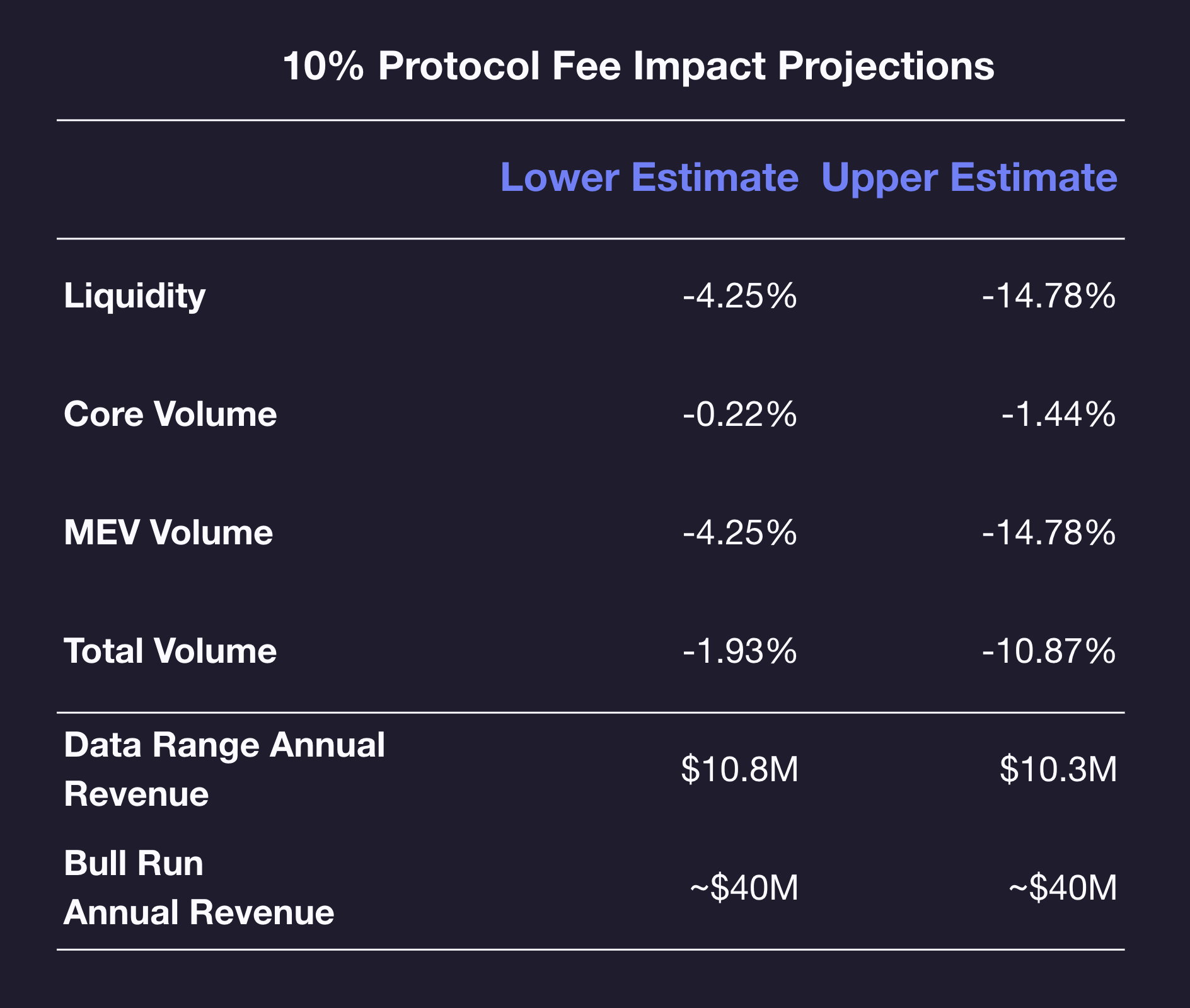
Core volume is relatively insensitive to fees, with less than 2% lost at a 10% protocol fee under our more conservative estimate. This is likely due to Uniswap's existing market share and substantial price improvement for swaps that are optimally routed to the target pools, which we described in the price execution analysis. Even a substantial decline in liquidity does not affect execution enough to re-route much core volume to competitors.

While we consider MEV volume to be much less economically meaningful than core volume, we recognize that headline DEX statistics do not differentiate between the two types. Thus, a significant drop in MEV volume may still be perceived as a serious economic issue by public opinion as it may cause a 10.87% loss in volume overall, despite causing minimal tangible harm. Though we do not attempt to quantify brand or PR impact in this report, we note that it may be an important qualitative factor for further discussion.

The table also shows estimates for annual revenue generated by the protocol fee. The "Data Range Annual Revenue" estimates are based on Uniswap's usage from August 2023 to January 2024, which is a period of lower volumes compared to historical months. Actual revenues could be substantially higher or lower depending on macro factors such as overall DEX trading volumes and crypto market prices. The "Bull Run Annual Revenue" estimates scale our volume projections to the peak market volumes observed in December 2021. One could scale the revenue projections further if this protocol fee were levied on all pools instead of just whitelisted pools: with a 10% protocol fee in the bull run scenario, we would expect $100M in annual revenue.

To better understand where the loss of core volume is occurring, we can look at these projections on a pool-by-pool basis. We would expect pools in the most competitive markets to losing more core volume, and pools that are dominant in their markets to lose very little.

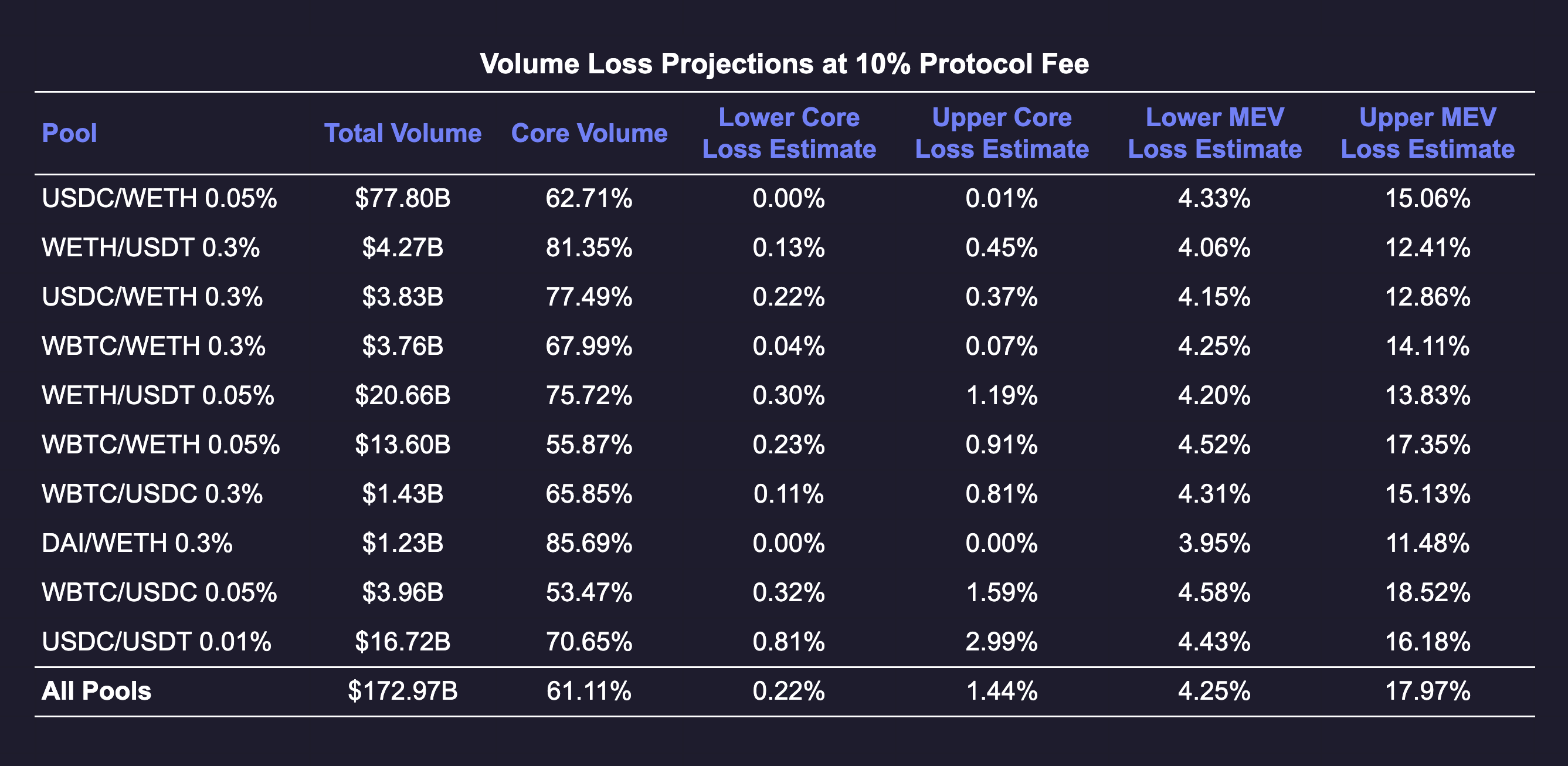
The table above shows the annualized volumes for each pool over the August 2023 to January 2024 period. We split each pool into MEV and core volume and show the impact figures for both categories. We can see that the core volume losses are quite small, and most significant in one highly competitive pool (USDC/USDT 0.01%). Since the USDC/USDT 0.01% pool has a well-known competitor (the Curve 3pool), we will now go through this case in detail to sanity check our results.

Model Validation

It may seem surprising that the impact of protocol fees on core volumes is fairly small. To illustrate why this is the case, we go through a sample of swaps routed to the USDT / USDC 0.01% pool and the competing Curve 3pool. The chart below shows the size of each swap and the price improvement that was obtained by routing to the optimal venue vs the competitor.

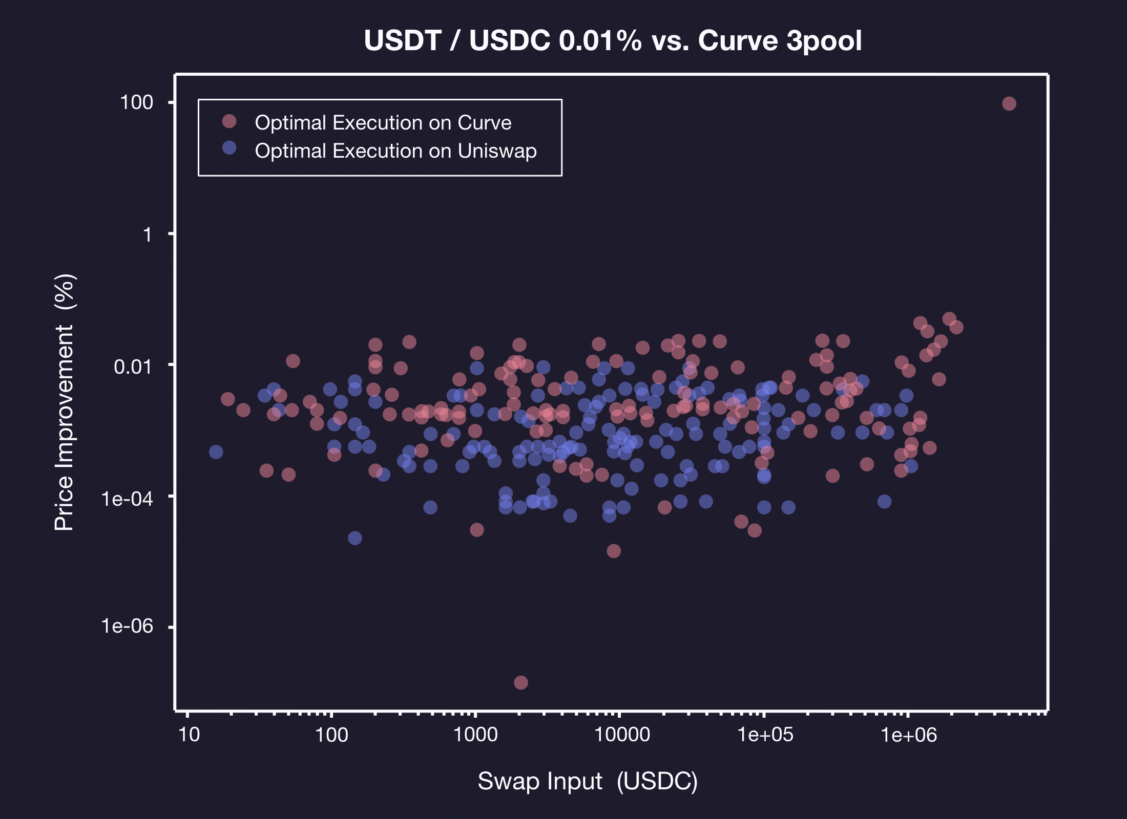
As expected for stablecoin pools, the price improvement is usually fairly small, and rarely exceeds 0.01%. The pools are highly competitive and receive comparable shares of swaps across a wide range of trade sizes.

The effect of a protocol fee in this picture would be to reduce the price improvement of Uniswap. If any Uniswap trades have their price improvement fall below zero, they would switch over to Curve due to re-routing to the optimal venue. The chart below shows this impact as the white line. Any purple dots below the line would be re-routed in the 30% protocol fee scenario.

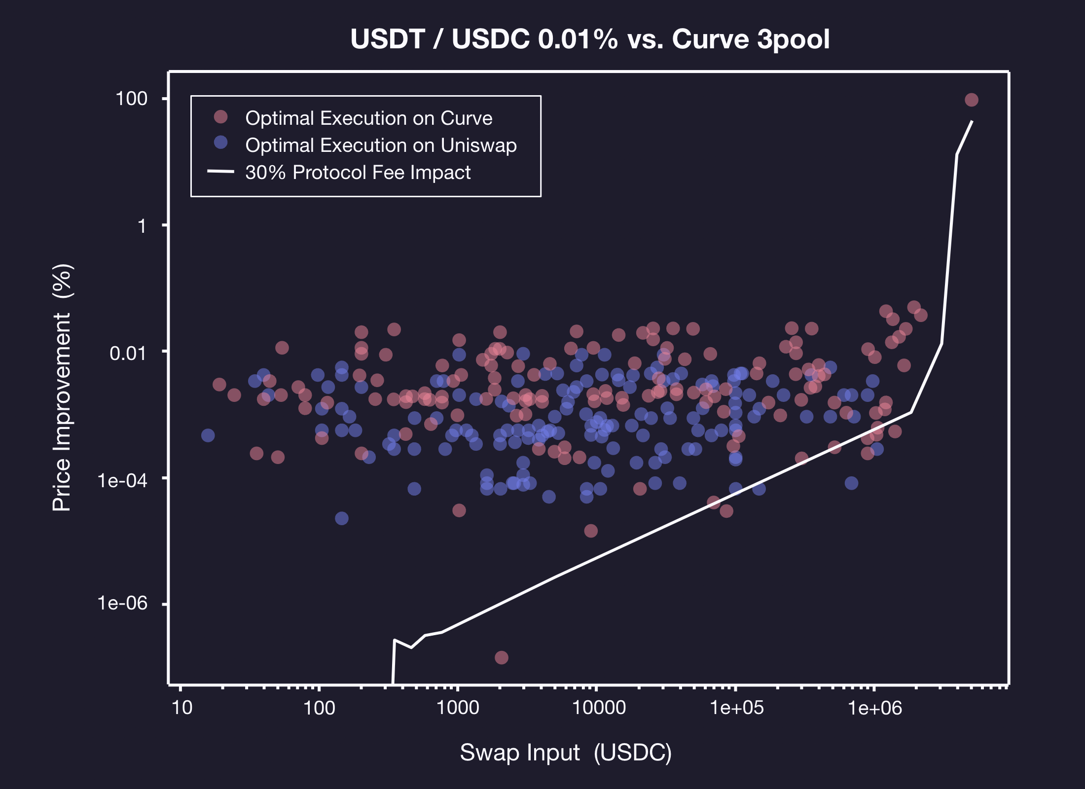
We note that for trades sizes below about $100k, the protocol fee impact is much smaller than the typical price differences between the venues. Between $100k and $1M, we note a few swaps that would be rerouted, which represent the core volume loss in the simulation. At very large trade sizes the fee impact starts increasing more quickly, as liquidity in the Uniswap pool starts to become a limiting factor.

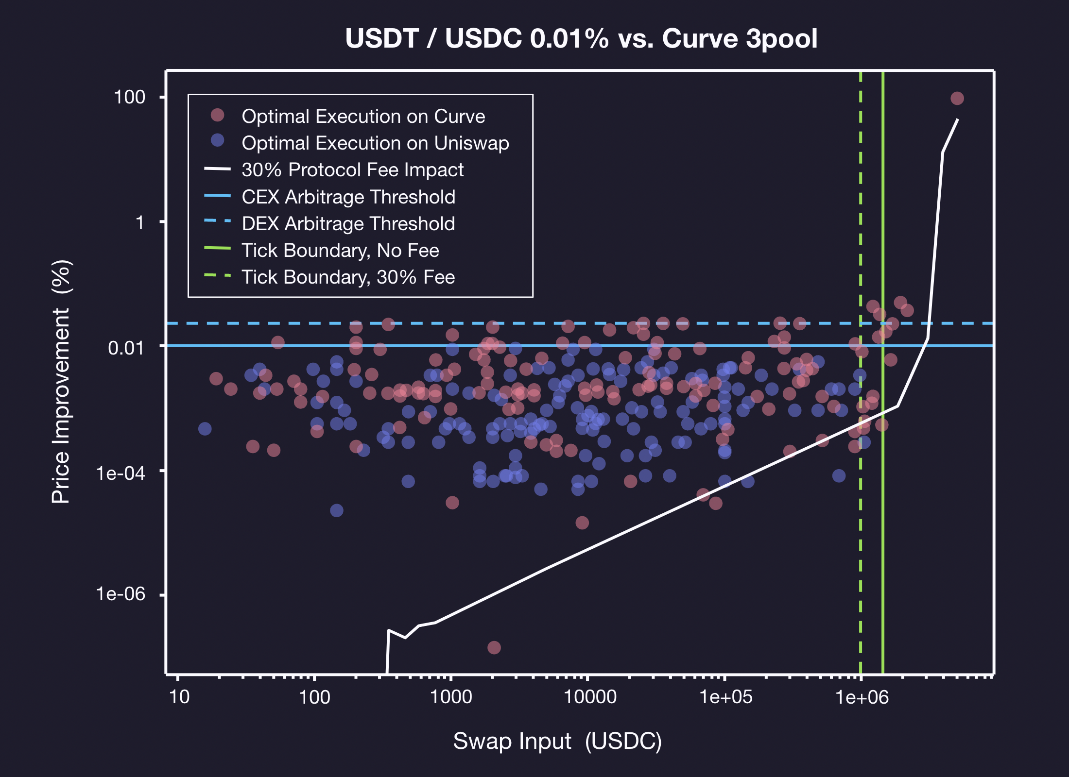
To set a benchmark for reasonable price differences, we add two blue lines for typical arbitrage thresholds in the chart above. Any differences above the solid blue line can likely be arbitraged against stablecoin liquidity on centralized exchanges, while the area above the dashed blue line can likely be arbitraged directly onchain. As expected, we see very few swaps executing above the blue lines, since such a large price improvement would be unsustainable in an efficient market. Below the blue lines there is not enough price difference to cover the operational and transaction costs of arbitrage, so this area is where most core volume ends up occuring.

The chart also includes the green lines which show the swap size needed to reach the tick boundary of the Uniswap pool. The solid green line is the actual average value over the sample period, and the dashed green line is adjusted for the protocol fee. This marks the point where slippage starts to increase notably in the Uniswap pool due to liquidity being a limiting factor. We note that the fee impact rises quickly after this point, as we would expect from the primary mechanism through which the fee affects the ecosystem being decreased liquidity. To the left of green lines, the fee impact is significantly less than one tick, which is also reasonable given the swaps here are occuring within a single tick bucket.

So we conclude that the low core volume losses are due to Uniswap’s strong existing market position and liquidity rarely being a limiting factor to core users, even at a fairly high 30% protocol fee. Having confirmed that the first-order model is reasonable, we can now move on to the flywheel case, which is our best forecast for what would actually occur.

Tradeoff Charts

To complete the review of results, we can visualize the pros and cons of a protocol fee discussed so far in a series of charts. We can plot the reductions of core and MEV volume for a given level of protocol fee, as shown for the core volume below. While Uniswap V3 only supports protocol fees ranging from 10-25% (specifically protocol fees of 1/10, 1/9, 1/8, 1/7, 1/6, 1/5, and 1/4), projections from outside of that range may be useful for designing future versions of the Uniswap protocol.

‍

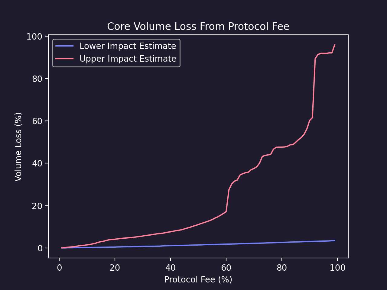
The core volume loss upper bound estimate is very non-linear, with the majority occurring at very high values of the protocol fee. On the other hand, the lower bound estimate is mostly linear and only reaches a maximum value of 3.5%. Reductions in yield as drastic as 50%+ are out of domain for our empirical elasticity model, so our lower bound estimates are likely overoptimistic for higher protocol fee settings.

At the extreme, a 100% protocol fee should result in a 100% loss of all volume, since such a DEX would be unable to retain any LPs. However, even for an extremely aggressive 60% protocol fee, the simulated DEX still retains substantial core volume under our more conservative perfect elasticity model. This once again highlights that liquidity is rarely a limiting factor for most of Uniswap's core users. Realistically, the protocol fee settings that are available for Uniswap V3 range from 10-25%. Within this range, the core volume loss curves are quite flat. This corresponds to the encouraging perceived core volume impact earlier in the analysis.

Switching to MEV volume, we see a very different picture:

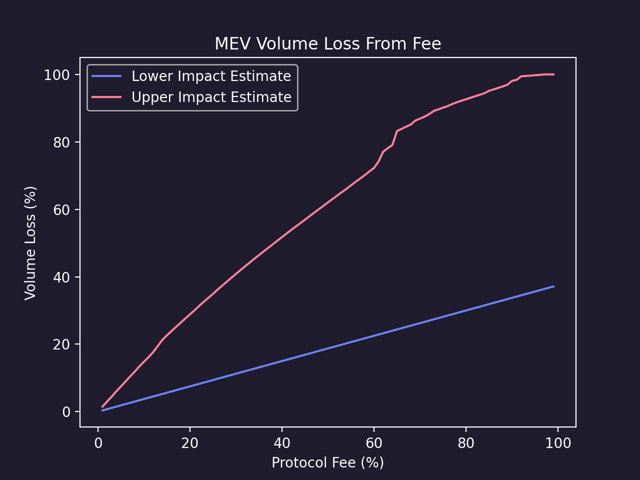
Due to the liquidity-sensitive nature of this volume and the linear relationship between the protocol fees, liquidity, and MEV volume discussed earlier, the impact is mostly linear. While the drop-off in MEV volume represents a minimal economic loss, it is still material in headline terms and needs to be considered for a full analysis of the tradeoffs.

Finally, we can look at the revenue generated by the protocol fee as the primary benefit of the tradeoff. The chart below shows the annualized revenue adjusted for the volume impact of the fee. At some level of the protocol fee, the volume loss under our upper impact estimate outweighs incremental revenue and leads to diminishing returns, similar to a Laffer curve seen in some tax revenue models.

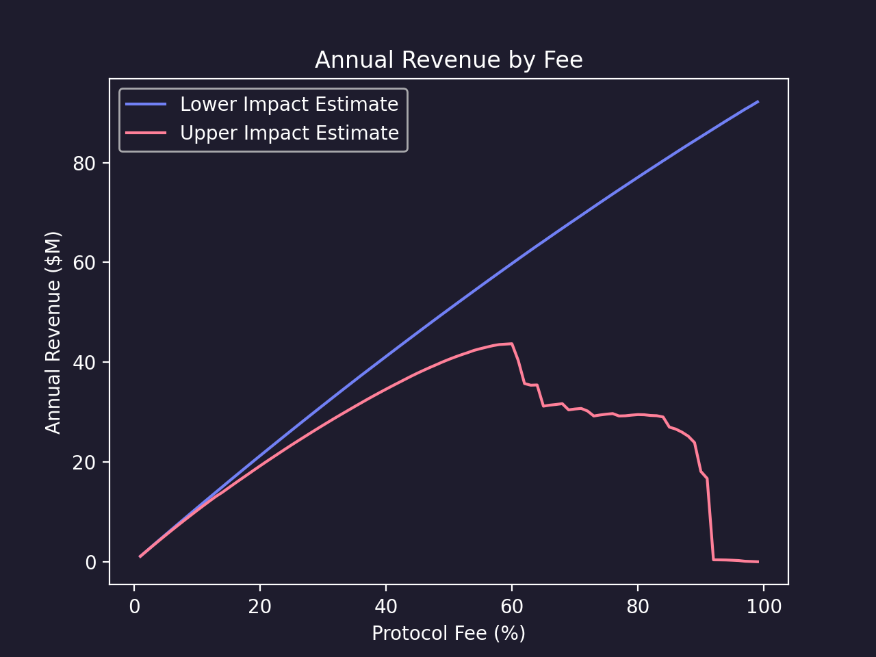
The revenue curve at higher values of the protocol fee depends significantly on the strength of the flywheel effect. Once core volume losses move into the steeper part of their impact curve, the downside risk of volume and revenue erosion starts to become more problematic. However, we note that for a viable 10-25% protocol fee, the revenue curves are fairly linear and far from the theoretical maximum. We conclude that a protocol fee in this range would be effective at generating revenue and is unlikely to suffer from diminishing returns due to core volume loss.

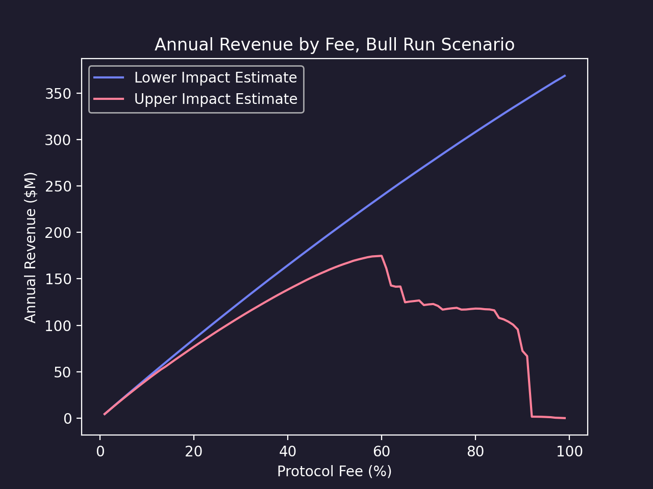
When interpreting the annual revenue chart above, note that this analysis was performed with swap data from August 2023 to January 2024, which had much lower volume than other historical time periods. If volume were at the peak levels seen in December 2021, then we would expect these revenue numbers to be around 4 times higher, which is illustrated in the figure below.

‍

Conclusions

The goal of this analysis was to evaluate the risks and benefits of protocol fees on Uniswap and evaluate their impact across different pools. We produced quantitative forecasts for liquidity, volume, and revenue, and now address the questions posed at the start.

1. Quantifying the potential benefits of a protocol fee

• How much revenue can a protocol fee generate?

The amount of revenue generated is a function of both the protocol fee set and the amount of trading volume. While we cannot predict macro factors that may affect the volume that is subject to the protocol fee, we can provide an estimate based on existing volume, adjusted for the volume impact of the fee.

Using our predictions of trading volumes at various protocol fees we are able to predict the amount of revenue generated. For revenue projections estimates we use the 3 month period from August 2023 to January 2024 as a reference lower bound and December 2021 as a reference upper bound for volume on Uniswap, assuming that the protocol fee is restricted to pools on the Uniswap Labs whitelist. We can consider 3 fee scenarios to illustrate the mechanics of the tradeoff, noting that these are chosen to highlight significant inflection points and are not necessarily practical options for Uniswap.

• Conservative (10% Protocol Fee) - A 10% protocol fee on the currently whitelisted pools would generate an expected $10.3M-$40M of annualized revenue.
• Flywheel Avoidant (20% Protocol Fee) - We find that the flywheel effect of reduced volume driving reduced liquidity only kicks in significantly at an ~20% protocol fee. Here we would expect to see about $19M-$72M in annualized revenue.
• Profit Maximizing (60% Protocol Fee) - Taking the effect of negative volume-liquidity flywheels into account we would expect to maximize protocol revenue at a 60% protocol fee driving an expected ~$43M-$160M in revenue. Note that a protocol fee this high is not supported by Uniswap V3, so this scenario is theoretical.

2. Quantifying the potential downsides of a protocol fee

• How much liquidity and volume would be lost?

The reduction in LP yields due to the protocol fee leads to an outflow of liquidity, which is the primary mechanism through which a protocol fee can negatively impact the rest of the ecosystem. We expect this is a roughly linear effect with increasing fees, so our projected outcomes for the three cases are:

• Conservative (10% Protocol Fee) - Reduces TVL by about 4.25-14.79%, roughly uniformly across the affected pools and tick distributions.
• Flywheel Avoidant (20% Protocol Fee) - Reduces TVL by about 28.46-28.85%, roughly uniformly across the affected pools and tick distributions.
• Profit Maximizing (60% Protocol Fee) - Reduces TVL by about 24.98-72.25%, roughly uniformly across the affected pools and tick distributions.

The impact of liquidity on trading volume depends significantly on the origin of the affected volume. Core retail and institutional users, which make up roughly half of the total volume on Uniswap, are not directly sensitive to liquidity, but rather indirectly through price execution quality. Our estimates for the impact of a protocol fee on core volume across all whitelisted pools are:

• Conservative (10% Protocol Fee) - Reduces core volume by about 0.22-1.44%, including minor negative flywheel effects.‍
• Flywheel Avoidant (20% Protocol Fee) - RReduces core volume by about 0.41-4.12%, including moderate negative flywheel effects.‍
• Profit Maximizing (60% Protocol Fee) - Reduces core volume by about 1.8-17.19%, including substantial negative flywheel effects. The likelihood of major negative flywheel effects that prevent further incremental profits increases quickly after this point.

On the other hand, MEV traders, who roughly make up the other half of total volume, are directly sensitive to liquidity. We project that reduced liquidity on Uniswap would reduce MEV activity by a proportionate amount, due to the smaller opportunities to profit from minor price dislocations. We then expect that a protocol fee would reduce MEV volume by the same percentages as TVL.

• Is there a threshold where fees create a major negative flywheel for users?

We estimate that a 10% protocol fee across all whitelisted pools would create a relatively minor flywheel effect. We also project that the point of diminishing returns, where the negative effects erode any incremental benefit of the protocol fee, occurs at protocol fees of about 60%.

3. Assessing the impact of a protocol fee across different pools

• Are some pools disproportionately affected?

The core volume losses are highly concentrated in a few pools with strong external competition. We especially note the USDT / USDC 0.01% pool, which competes closely with other stablecoin pools, such as the Curve 3pool. We estimate the USDT / USDC 0.01% pool would lose 0.81-2.99% of its core retail and institutional volume at a 10% protocol fee, compared to a 0.22-1.44% volume loss for the average pool.

Losses in liquidity and MEV volume are more widespread, as we expect them to reflect a uniform reduction in activity proportional to the protocol fee.

Overall Recommendation

If the Uniswap governance community were to consider implementing protocol fees, Gauntlet recommends an incremental approach to rolling them out. This should begin with a low fee on select pools, followed by an extension to additional pools and a gradual increase in the fee on existing ones, in order to validate the projections presented in our report. Under current market conditions and during an upswing, a conservative fee on carefully selected pools would generate a significant amount of revenue with a limited impact on non-MEV volume.

The community choice of whether or not to institute a protocol fee comes down to whether or not the long-term revenue gained outweighs the losses in volume and liquidity.

Our analysis shows that the losses to TVL and toxic MEV volume may be significant with even a conservative fee switch. Still, we expect the impact on core, non-MEV volume to be very minor under all but the most extreme fees. The only means to identify if a fee switch is an optimal strategy for the Uniswap DAO and protocol community is to perform calculated experiments with a live fee switch, which Gauntlet is keen to help craft.

Last updated 2/27/2024